一维傅里叶变换

文中公式渲染不正确时请刷新网页

什么是傅里叶变换

笔记

Fourier Transform (FT)

$$
G(f)=\int_{-\infty}^{\infty} g(t) e^{-i 2 \pi f t} d t=F{g(t)}
$$

Inverse Fourier Transform

$$
g(t)=\int_{-\infty}^{\infty} G(f) e^{i 2 \pi f t} d f=F^{-1}{G(f)}
$$

其中，$i=\sqrt{-1}$，表示复数虚部

单位

Temporal Coordinates, e.g. $t$ in seconds, $f$ in cycles/second

$$
\begin{array}{rrr}G(f) & =\int_{-\infty}^{\infty} g(t) e^{-i 2 \pi f t} d t & \text { Fourier Transform } \\ \\
g(t) & =\int_{-\infty}^{\infty} G(f) e^{i 2 \pi f t} d f & \text { Inverse Fourier Transform }\end{array}
$$

Spatial Coordinates, e.g. $x$ in $\mathrm{cm}, k_{x}$ is spatial frequency in $cycles/ \mathrm{cm}$

$$
\begin{array}{lc}G\left(k_{x}\right)=\int_{-\infty}^{\infty} g(x) e^{-i 2 \pi k_{x} x} d x & \text { Fourier Transform } \\
g(x)=\int_{-\infty}^{\infty} G\left(k_{x}\right) e^{i 2 \pi k_{x} x} d k_{x} & \text { Inverse Fourier Transform }\end{array}
$$

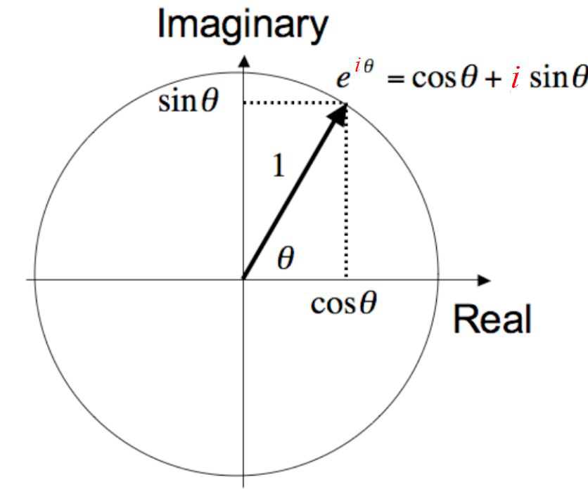
Euler’s Formula

$$
\begin{aligned}
&e^{i \theta}=\cos \theta+i \sin \theta \\
&z=x+i y=|z| e^{i \theta}
\end{aligned}
$$

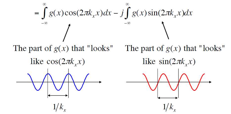
根据欧拉公式将傅里叶变换展开：

$$
\begin{aligned}
G\left(k_{x}\right) &= \int_{-\infty}^{\infty} g(x) e^{-i 2 \pi k_{x} x} d x \\
& = \int_{-\infty}^{\infty} g(x) \left(cos(- 2 \pi k_{x} x) + i sin(- 2 \pi k_{x} x) \right) d x \\
& = \int_{-\infty}^{\infty} g(x) cos(2 \pi k_{x} x) d x - i\int_{-\infty}^{\infty} g(x) sin(2 \pi k_{x} x) d x
\end{aligned}
$$

Spatial Coordinates, e.g. $x$ in $\mathrm{cm}, k_{x}$ is spatial frequency in $cycles/ \mathrm{cm}$

一维傅里叶变换的Python实现

来源：python实现一维傅里叶变换和逆变换_bilibili

代码如下：

import numpy as np
import matplotlib.pyplot as plt

'''
离散点的时域分析
'''

M = 1000
test_x = np.linspace(0, 4 * np.pi, M)
test_y = np.zeros(test_x.size, dtype=complex)

for i in range(1, M + 1):
    # y是M个不同幅度的正弦序列的叠加
    test_y += 4 * np.sin((2 * i - 1) * np.pi * test_x) / (np.pi * (2 * i - 1))

# Fourrier transform
# test_y_fft = np.fft.fft(test_y)
fu_array = np.zeros((M, M), dtype=complex)
fu_array = np.array([[test_y[t] * np.exp(-1j * 2 * np.pi * u * t / M)
                      for t in range(test_y.size)] for u in range(test_y.size)])
FU = np.array([np.mean(fu_array[u]) for u in range(M)])
FU1 = FU.reshape((1, -1))
# print(u_array)
print(fu_array)
print(FU1.shape)

# Inverse of Fourier transform
# test_y_ifft = np.fft.ifft(test_y_fft)
# print(test_y_ifft)
fx_array = np.zeros((M, M), dtype=complex)
fx_array = np.array([[FU1[0, t] * np.exp(1j * 2 * np.pi * u * t / M)
                        for t in range(M)] for u in range(M)])
FX = np.array([np.sum(fx_array[t]) for t in range(M)])
FX1 = FX.reshape((1, -1))

plt.figure(figsize=(12, 8))
plt.subplot(211)
plt.title('Original Signal')
plt.grid(linestyle=':')
plt.plot(test_x, test_y, 'r-', label='y')
plt.legend()

plt.subplot(212)
plt.title('Inverse of Fourier Transform')
plt.grid(linestyle=':')
plt.plot(test_x, FX1[0], 'b-', label='y_new')
plt.legend()
plt.tight_layout()
plt.show()

附原视频：